The page has been designed and written by Ayumi Ozeki ozekia@gmail.com
go to home http://ayumi01.s3-website-us-east-1.amazonaws.com
Cloud based simulation engine
This white paper describes the reengineering opportunities for
financial simulation engine utilizing Amazon SQS, AWS Lambda, Amazon
ElasticCache, and Amazon Redshift. Among varieties of cloud benefits, faster
results availability and pay-as-you-go model have unique implications to
simulation engine usage.
First let’s examine typical scaling technique used for simulation
engine. If you want to skip intro and go right to the Amazon Lambda based new
architecture section, click here.
Instant simulation result?
Generally speaking running simulation takes time to prepare, to run,
and to compile results. Vertical scaling (use of more powerful computer) and
horizontal scaling (adding nodes) will help completing the tasks faster. If we
can achieve performance gain where 10 times nodes mean 10 times faster job
completion, that suggests under the pay-as-you-go model it should cost the same
while achieving fastest time to delivery. When diminishing return on additional
node begins to materialize, however, the idea of provisioning massive nodes to
get the result instantly might not work too well. Considering the fact that
simulation involves processing the same routine as many times as the scenario
count with different simulated variables, such scaling conceptually works very
well, except there is a limit to this in reality.
Issues arise as scheduler gets busier and each node starts to have
varying degrees of the resource usage – i.e. increasing the node 10 times does
not mean 10 times faster unless each node uses identical resources, execute
same way, each task completion time being identical, and there is constant
coordination overhead. This is not the case. Many techniques exist to make it
efficient but perhaps the fundamental limitation is in its architecture of
distributing chunk of work to each node. Such “chunk of work” as a whole can be
quite complex, resulting in diverse resource usage across nodes. Scheduler gets
very busy finding available node to assign jobs and as such it gets very busy
as the node count gets higher.
The sections that follow will focus on end-of-the-day simulation-based
risk calculation as the basis of the discussion. Other types of the usage are
actually similar in architecture fundamentally. Let us first review the general
processes.
End-of-the-day financial risk calculation
The processes typically
happen in the following steps:
1.
Sourcing customer data
1.1.
Portfolio details
1.2.
Reference data such as customer’s risk rating and legal attributes that
affect risk attributes
2.
Gathering market factors
2.1.
Observable market data
2.2.
Derive additional data such as correlation and historic volatility from
observables
3.
Creating scenarios
3.1.
Simulate observable market factors
3.2.
Derive additional market factors from simulated ones
3.3.
Further derive the state of transaction set and reference data
4.
Pricing portfolios per scenario
5.
Determining expected value and stressed values of varying degrees based
on the scenarios
The most computationally intense part is step 4. Since there is no need
to complete it in a synchronous fashion it presents a great distributed
parallel processing opportunity. One possible distributed architecture is to
assign a task to a node in completing portfolio valuation per specific
scenario. A node may be assigned to do the routine for multiple scenarios –
i.e. doing the similar calculation routine repeatedly. This table helps
illustrate ways a task distribution can be designed.
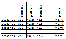
For example, a node may be
assigned:
-
By row slicing
o One or more scenarios and
valuation of all portfolios
o For a scenario valuation of
subset of portfolios
-
By column slicing
o Valuation of one or more
portfolios across all scenarios
o Valuation of one portfolio
under subset of scenarios
The idea is slicing the valuation needs by portfolio and by scenario,
and assign to each node accordingly. Again, asynchronous processing is
perfectly fine no matter how it is sliced. Before proceeding to the step five
to determine portfolio risks, all the valuation must be completed.
For a node to complete a
whole pricing of a portfolio – i.e. determining v(x, y) - it involves the
following computation steps:
1.
Given a set of instruments in a portfolio, determine necessary pricing
functions
2.
For each instrument that must be priced, determine market factors
required to price
3.
Retrieve unique set of market factors from a scenario, and price all
instruments in a portfolio
4.
Determine a portfolio price for the scenario
Distributed nodes typically perform all these steps by loading all
necessary pricing functions and required market factors. The node further runs
multiple valuation per scenario. As illustrated before, the job distribution by
portfolios and/or scenarios seems quite simple except across nodes, substantial
overlap in resource demands exist. For example, by scenario job distribution
means all nodes will load the identical portfolio data and pricing libraries.
In contrast, by portfolio job distribution means identical scenario data loaded
to all the nodes. Either way it appears inefficient.
Further decomposition below what has been illustrated is certainly an
idea – i.e. a node that specializes in pricing specific instruments, for
instance. The problem is now the scheduler. Each pricing engine requires
different sets of inputs and computation time requirement differs. A node that
specializes in FX forward pricing may finish all the work before more complex
credit default swap (CDS) engine has not even finished 10% of the work. A
scheduler can then assign next sets of CDS jobs to this idle node that used to
process FX forward. This process gets very complex and eventually becomes
inefficient as node count increases. It is inevitable idle resources pile up,
diminishing the return on additional node.
The prior section provided an example of how decomposition of processor
below portfolio valuation per scenario ends up creating scheduling challenges
and introducing diminishing return on additional nodes. This is where AWS
Lambda comes in.
AWS Lambda is a unique serverless architecture that is not available as
on-premise solution. You can’t just buy Lambda package and install on your
server. The fact that AWS Lambda executes code only when needed, scales
automatically, and as usual only pay for the usage while AWS takes care of
various underlying administration, it sounded like a magic wand in solving
typical simulation engine architecture limitations. Theoretically a task and
computational needs assigned to a node can be broken into multiple AWS Lambda
functions, and each function can be run to the maximum concurrent run limit.
This sounds akin to achieving zero idle node.
In reality there is an AWS Lambda concurrency limit, and thus you can’t
let million AWS Lambda function run at the same time and finish the simulation
instantly. However, you can request the concurrency limit increase and it is
worth exploring new architecture by combining additional AWS features and
services. From an architectural point of view, it provides an attractive
opportunity to decouple specific computation task from resources that happened
to be provisioned by an end user.
The following specialized
sets of AWS Lambda functions should be considered:
1.
Market
factor generators, lm
2.
Scenario
generators, ls
3.
Pricing
engines, lp
4.
Aggregation
engines, la
5.
Risk
determinants, lr
Not surprisingly these functions are aligned to what are listed in the
prior section as to how simulation preparation and runs take place. Further,
each set must be completed before proceeding to the next. However, within the
set, asynchronous processing and thus scaling will reduce total processing
time. One thing missing is the customer data sourcing part. This process may
not benefit much from AWS Lambda since such job is typically in persisting once
and reading many times, something typical ETL and data warehousing techniques
can already do a good job. Amazon Redshift sounds perfect for this as it is
designed for OLAP. But the rest of the processes are the core of the time
consuming simulation engine that can be architected very differently than
typical distributed simulation engine.
Besides concurrency limit, there is also a time limit. Based on the
understanding of each specific processing needs, it’s actually hard to imagine
a specialized AWS Lambda function for financial simulation to exceed time limit.
The reason the whole simulation engine takes very long time is driven by
massive number of repeated processes, not really one specific atomic task
taking very long time. Considering the way above AWS Lambda functions are
designed, the behavior should be about the same; each function call should
finish instantly but need to run so many times.
Since AWS Lambda supports dozens of event sources, scheduling of
function calls can be designed in many ways. Amazon SQS for example is one
candidate to invoke functions where within each set of the functions listed
above the job can be completed asynchronously. Since Amazon SQS supports
message attributes that supports string and numeric data type, additional data
can be used by the listener. This can further manage the effective distribution
of the computation tasks. Let’s examine deeper each function.
Considering the subsequent OLAP needs, all the generated data will be
persisted in Amazon Redshift since the usage is write once and read many times.
lm - market factor generators
Preparing end of the day market factors might not be the most
computationally intense task. Further this job needs to be run just once,
unlike processing needs that varies depending on the scenario count. Having
said that there are still opportunities to introduce parallel processing as
it’s not that there is only one specific processing rule that can create all
derived factors. For example computing correlation is totally different from
determining historic volatility of observable market data. Yet the computation
of volatility and correlation may be based on the same data. Therefor
developing specialized AWS Lambda function designed for varieties of market
data preparation is certainly not a bad idea at all. If not for significant
performance boost but at least achieves good component architecture.
ls - scenario generators
Depending on how scenario generation rule is decomposed, there are
varieties of opportunities in creating scenario generators. Similar to the
table shown in prior section (scenario vs. portfolio), scenario generation can
take place via parallel processing. For example, market factors can be grouped
so that across such groups zero correlation can be assumed. Then this presents an
opportunity for asynchronous parallel processing – i.e. invoking many ls at the same time to
complete the task instantly. There’s also a way to logically break into pieces
for more parallel processing. As discussed before, when Amazon SQS is used as a
scheduler, it can include additional attributes. When the attributes are
created in a controlled fashion, then it can further aid in decomposing a
routine into pieces. Consider the following code: for i=1 to 100; process f(i);
next i. Breaking this into two pieces where: 1) for i=1 to 50; 2) for i=51 to
100. It may / may not work but if an Amazon SQS message includes 1/50 vs.
51/101 values, then the function can be run in parallel. Depending on the
specific design of scenario generation there are ample opportunities to run
various ls function in parallel.
lp – pricing engines
Developing pricing libraries and reusing them across distributed nodes
is nothing new. Conceptually this lp function is no different. But the
environment in which this is run is so different than, say invoking FX pricing
function within code run on EC2, it makes a huge difference in efficiency. An
infrastructure that consists of many nodes is as if full of having many bloated
nodes. The benefit of AWS Lambda architecture is expected to be the most
significant from the pricing part. This is because due to the AWS Lambda driven
architecture, the entire pricing part of the simulation engine can be done
across all scenarios and portfolios in an asynchronous fashion. If there is no
concurrency limit at all, theoretically this part, which is the most time
consuming, can finish instantly by running infinite number of lp at the same time.
Consider the following table that shows various instruments per
portfolio, and pricing needs across all scenarios:
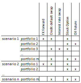
While traditional distributed computing design can take each “x” mark
and let the scheduler distribute across nodes, it gets very busy quickly and
idle nodes persists. An attempt to decouple components increases scheduler
overhead whereas less scheduler demands creates complex (coupled) big job
assigned to a node that has diversity in resource demands and in completion
time.
AWS Lambda driven way of pricing, however, all “x” marks in the above
table if not constrained by concurrency run limit can be completed
simultaneously without any coordination (scheduling) needs. This is because
each “x” computation has no synchronization needs within pricing step.
Especially that this pricing portfolios across all scenarios is almost always
the most time consuming part of the financial simulation, this could be a major
game changer.
Let’s not also forget that Amazon ElasticCache will aid performance
boost even more. Each specialized function has specific sets of market data
needs, and AWS Lambda is ready to take advantage of Amazon ElasticCache. FX
forward lp has no need for stock market data and oil future lp only needs to worry about
discount rate and related commodity factors. Thus FX forward lp can rely on readily
available FX data in Amazon ElasticCache for its very specific FX pricing
needs.
la – aggregation engine
After all lp complete the jobs, it’s time for the next step - la to begin the process of
aggregation. This process is nothing but aggregating all instruments in a
portfolio to determine the portfolio value for each scenario. Total computation
required depends on number of instruments, portfolio count, and scenario count.
la can
do the bare basic of determining all of portfolio values across all scenarios.
This part again can be done asynchronously, and thus la can be invoked many times
concurrently, reading the data from the Amazon Redshift, to finish the job
extremely quickly.
lr – risk determinants
Typically for the purpose of risk analysis and reporting, expected and
stressed values are produced. Each risk reportable is based on portfolio value
per scenario – the same sets of data produced in the prior step, except how to
use them is different. As such various lr can be defined and they can all run
concurrently to finish the job as fast as possible. One lr will compute expected
portfolio value (average of portfolio value across all scenarios) whereas
another lr will pick 95th percentile and 99th percentile
worst case scenario.
Post processing analysis
All the results, whether a price of an instrument under a specific
scenario, or a portfolio value under another scenario, should be persisted in
Amazon Redshift for subsequent OLAP analysis. As with transaction data, as
various AWS Lambda function computes, it’s all write once and read many times
case. Combined with trade details already in Amazon Redshift, combination of
simulation results also in the same environment enables enormous OLAP analytics
opportunities. For example, tracing of specific one or more instruments or
portfolios across time and underlying factors, and further across scenarios,
are all part of rather plain vanilla OLAP activities. Perhaps after a month or
whenever the OLAP needs decline, data can migrate to Amazon S3, and eventually
Amazon Glacier.
In addition the data whether in Amazon S3 or in Amazon Redshift
presents another analytic opportunities with various Machine Learning (ML)
tools. In order to do ML with financial transactions and market data, you would
have to have the same sets of the data anyway. The whole simulation process
already created such sets.
Practical use
This brand new architecture brings not only decoupling benefits but
also most importantly considerable performance boost. In a way AWS Lambda
architecture makes it a lot closer to achieve the following: today it takes 10
resources 10 hours; tomorrow we run 10,000 resources and finish in 3.6 seconds,
still costing the same in the end.
The idea of eventuality where simulation result becomes instantly
available is totally revolutionary. Today over-night risk processing is typical
and during the day, traders rely on approximation to do their job. Often enough
sensitivity factors are also produced over-night so that during the day without
instant simulation capability, delta and gamma are used to determine
anticipated risk (to be proven after another over-night batch). If the
simulation result is available instantly, however, a trader would input
prevailing rates and gets the results, which will be the most useful.
Given the pay-as-you-go model, a trader will have a discipline in
utilizing such capability. Instead of running one simulation request to another
(since it’s instantly available), the traders are told by finance that each run
cost specific certain amount. This is where detailed cost report by account and
specific cloud resources come in handy. Unless economically makes sense, it
must be discouraged to run whatever it costs to run simulation. The specific
cost will be explicit. Over a very long time, however, the cost will be so low
and the speed is so fast, the simulation engine becomes another cheap utility.
In the U.S. all the major banks are required to submit capital plan
every year per so called CCAR requirements. The deadline for annual submission
does not move yet scenarios regulators release is often delayed. When running
faster is all about provisioning more resources, the cloud architecture and
certainly AWS Lambda simulation architecture is extremely attractive, assuming
scale out is as effective. In a typical scenario, when time to submission
shrinks, planned simulation run will be cut back as it becomes physically
impossible to run very time consuming simulations. The architectural changes
that enables time to complete and pay-as-you-go will dramatically change the
planning and execution.
Perhaps not so fast
For those who consider such AWS Lambda driven reengineering is a
considerable undertaking and thus less dramatic upgrade, or intermediate
reengineering, might be desired. In this section such intermediary architecture
that is a stepping stone to the AWS Lambda based architecture is discussed.
In fact the following steps could be considered a complete cloud
migration strategy; each step bringing in material benefit while at the same
time such staged approach mitigates the risk of huge waterfall that could
break.
1.
On-premise architecture to be migrated to cloud with as little
modification as possible
2.
A job scheduler is replaced by Amazon SQS, and Auto Scaler manages EC2
instance needs
-
Alternatively, or as the next step following SQS based architecture,
develop Elastic Beanstalk application
3.
Jobs performed by EC2 to be replaced by AWS Lambda functions
The first step of just migrating to cloud with little modification
automatically benefits in cost saving. It’s also quite likely to see some level
of performance boost by adding nodes during peak time. The second step is an
intermediary step before full serverless architecture kicks in. Yet this
already has a benefit of decoupling, and benefit of each additional node is
expected to be more than step 1. This is because each node is constantly
processing and as soon as it is done with the job it takes the next available
SQS message and keeps running. It’s quite possible to have significant number
of EC2 instance to be created and concurrent message consumption can be
achieved. Before stepping up to the final stage, Elastic Beanstalk based
application might be an easier step before going to AWS Lambda based. At least
you can take full advantage of managed services. The final step of AWS Lambda
driven architecture is akin to eliminating EC2 from the picture in the second
phase.
My thoughts
Varieties of cloud based simulation documents seem to focus on
migration of existing distributed architecture to cloud. That does have huge
benefits. When seniors learn that on-premise servers are 100% utilized a few
days a month and the rest of the month the usage is under 10%, they have real
hard time keeping all the boxes online doing nothing most of the time. This is
a classic cloud migration benefits.
It turns out at AWS re:Invent 2017, “AWS Lambda for Financial Modeling” talks
about traditional High Performance Computing (HPC) and AWS Lambda based
architecture, which in principle the same as what is discussed in this white
paper. However, this re:Invent presentation talks nothing about specific steps
such as market data preparation, scenario generation, etc. I found the
presentation to be a great intro and thus it is encouraged to watch.
This AWS Lambda based simulation architecture is an elegant one that is
aiming towards massive parallelism that in the end does not cost any extra than
running less slowly. I would like to believe it is a matter of time where we
pay for simulation and the result is available instantly. That certainly
revolutionizes risk management entirely.
The
last update: 12/25/2018
The
page has been designed and written by Ayumi
Ozeki ozekia@gmail.com
go
to home http://ayumi01.s3-website-us-east-1.amazonaws.com